
The stacks of white rows can dull your senses. Shading every other row in Excel can produce a wonderful contrast between these white rows and brighten your Excel experience.
There are many in-built color patterns and schemes you can use to shade your Excel data. A conditional format is the easiest way to apply these color schemes.
In this tutorial, we will discuss how you can use conditional formatting to apply shade alternating lines.
Shading Every other Row in Excel ( Using Conditional Formatting)
1. Open the Excel Document containing your data.
2. Select the range of cells you wish to shade.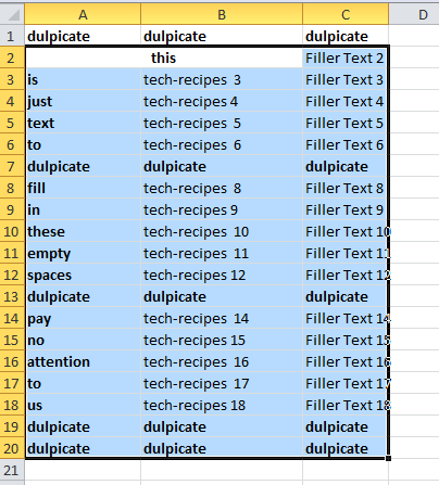
Note: Select the entire range, not just alternate rows.
3. In the home tab, tap Conditional Formatting.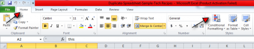
4. Select New Rule… from the drop-down menu.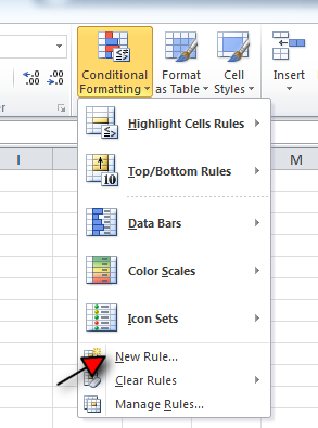
5. Select “use a formula to determine…” as Rule type. It’s the sixth one.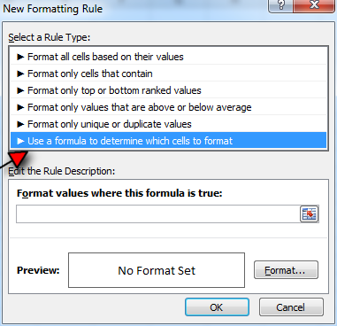
6. Insert formula: MOD(ROW(),2) in the space below Edit this Rule Description.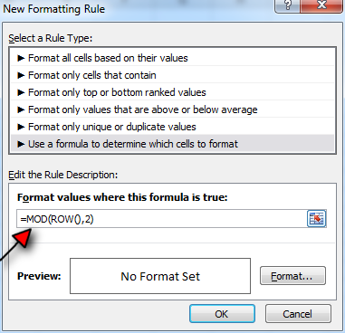
7. Tap Format in the same window (adjacent to preview).
8. Select the fill tab.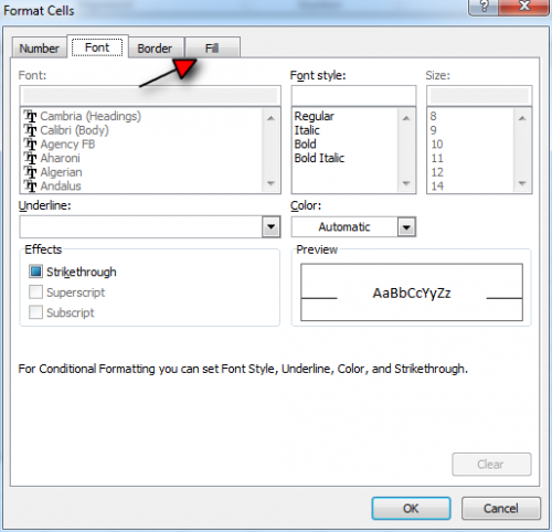
9. Select the color you want your alternate rows to have and tap OK.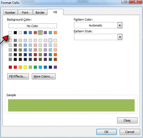
10. Tap OK again.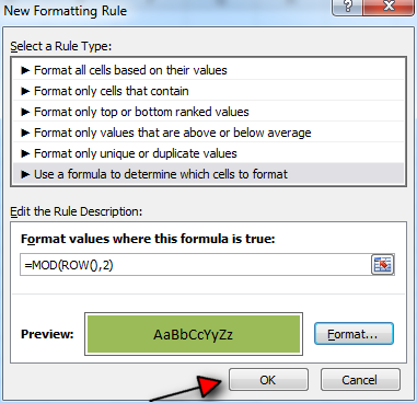
11. Voila! your alternate rows are here.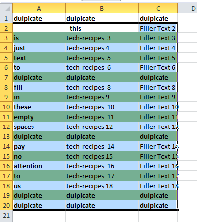
Read a Similar Excel Tutorial: How to Create a Pictograph in Excel
Understanding the Alternate Row Shading Formula
If you’re interested in the science behind the Excel Function: MOD(ROW(),2), here’s a simple explanation.
The MOD and ROW function deal with the remainder of division and row number respectively. For example, for the ninth row, the formula MOD is (9,2). 9 is divided by 2 (5 times) to extract a remainder of 1. Whereas the for the tenth row, MOD is (10,2). 10 divided by 2 six times is 0. Apply this formula to all rows and only MOD for odd rows returns as 1, and consequently, they are shaded.
Youtube Tutorial
Following text and picture instructions isn’t for everyone. Some people prefer Youtube tutorials to understand the process that goes into shading every other row in Excel.
For your further convenience, below is a video tutorial explaining exactly that. The version of Microsoft Excel used in this Youtube tutorial is Excel 2013. However, the steps remain identical across all versions of Excel, including 2013, 2016, Excel Online and the latest 2019.

