
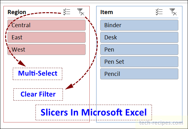
Slicers provide an interactive way to filter the data with list and buttons. It shows which filters have applied and a list of possible values in a presentable manner. Using the existing dropdown filter which lacks showing all the possible values on the sheet for presentation. Strongly recommended the feature Slicers when presenting data analysis to customers and stakeholders with an interactive dashboard.
1.
Slicers in Microsoft Excel
1. Interactive ways to show a list of values and buttons for filter.
2. Smart and easy way to filter data in tables and pivot tables.
3. Single or multiple values selectable.
4. Cascading of slicers updates itself based on the filter selection.
2.
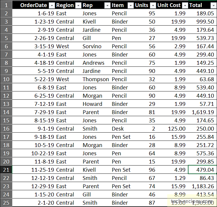
Data Set
Following data set used to demonstrate slicers in Microsoft in this post. Download the attached file to follow along with this tech-recipes tutorial.
3.
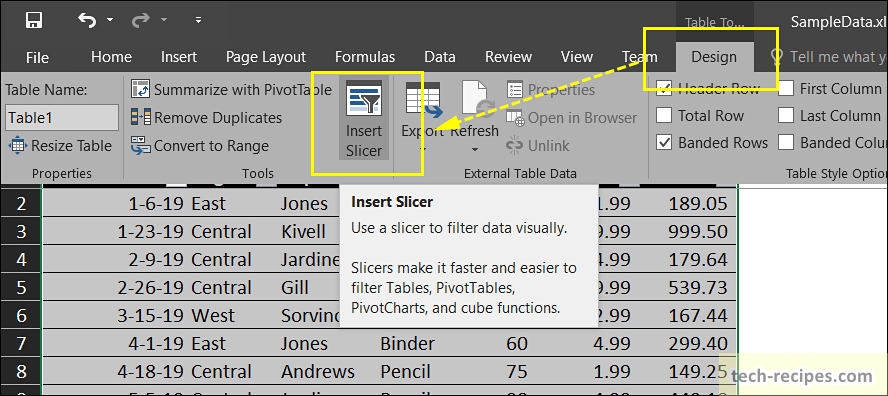
Insert Slicer – Excel Table
1. Select any random cell in the Microsoft Excel table and go to the Design tab.
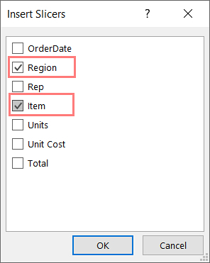
2. Click on Insert Slicers.
3. Select a list of columns to create multiple slicers.
4.
Insert Slicer – Excel Pivot Table
1. Select any random cell in the Microsoft Pivot table and go to the Analysis tab.
2. Click on Insert Slicers.
3. Select a list of columns to create multiple slicers.
5.
Filter Slicers In a Table – Single Selection
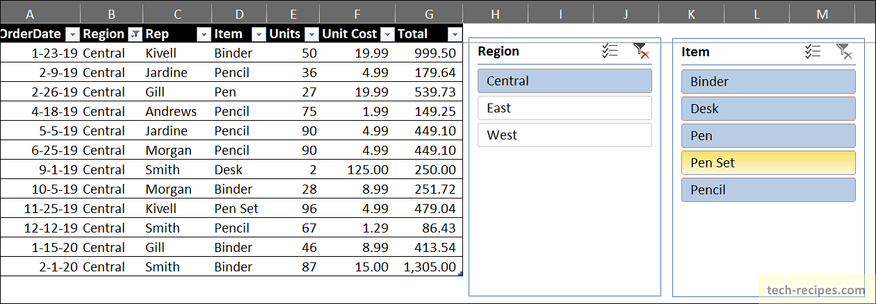
In the following image, a single filter Central in Region slicer is selected to filter out the data.
5.
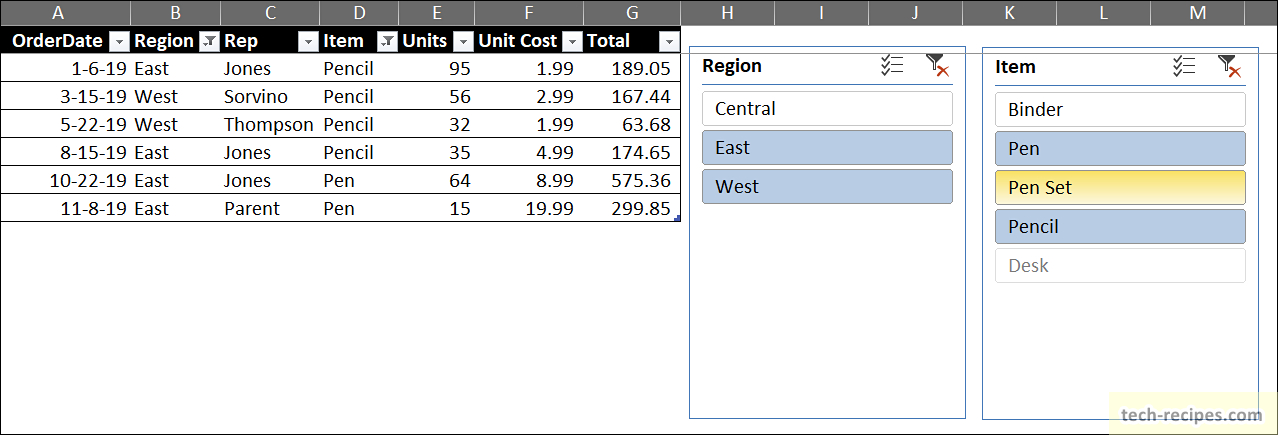
Filter Slicers In a Table – Multi Selection
Here following the figure, multiple values are selected. Hold the SHIFT key and select multiple values from slicers list.
6.
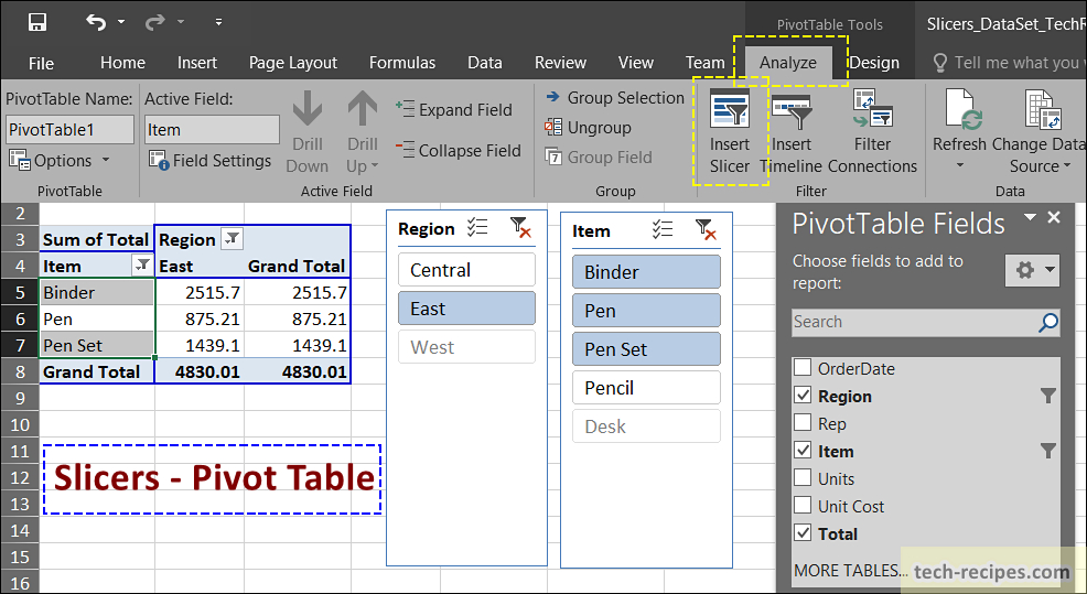
Filter Slicers In a Pivot Table
Similar to the table we can filter out data using slicers in the Pivot table. Single selection & multi selection works here too. Slicer needs to be inserted from the Analysis tab in case of Pivot tables.
7.
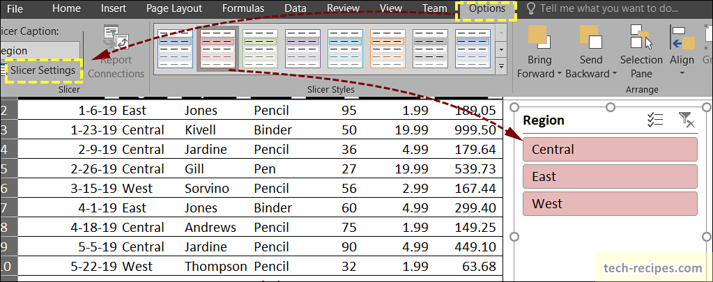
Slicers – More Customization
Numerous customization options are possible to added slicers. Select the slicer and navigate to the Options tab. We can change the colour, height, weight from the options tab. Click on Slicers Settings in Options tab to decide the Order of items in slicers list and rename the Slicers title head.
Summary
In a nutshell, we have learnt to use Slicers to create interactive filters and dashboard. This shows the data and filters in a more presentable manner to customers and stackholders. Data analysis becomes easy to present to larger audience with ease. If you like this post you may read more on Microsoft Excel on Tech recipes.
1. How to Convert Your Excel Spreadsheets to Google Sheets
2. How to Freeze Panes in Excel — Lock Columns and Rows
3. How to Remove Duplicates in Excel
4. How to View Excel on Two Monitors

