
Pie chart is perhaps the most common method to represent data quantitatively. It shows how much of a certain category contributes to the overall population. It is also used to compare one value set from another, but only if the values are too large or too small. Close values are compared best by a bar graph. A pie chart comprises of slices, each of which represents a given value in the form of numbers, percentages, series’ names and other forms. From advanced chart labeling to simple worksheet tab options, Excel lets users create wholly customizable pie charts from myriad design options. The experience is both creative and professional.
Step-by-Step: How to Create a Pie Chart in Excel
Getting Started: Naming Your Pie Chart
1. Open your Excel workbook.
If plain white feels like a dull background for your pie-chart, you can also create it against a background image in Excel.
2. Enter your data.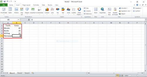
3. Select the first cell and drag cursor till the last cell to select whole data.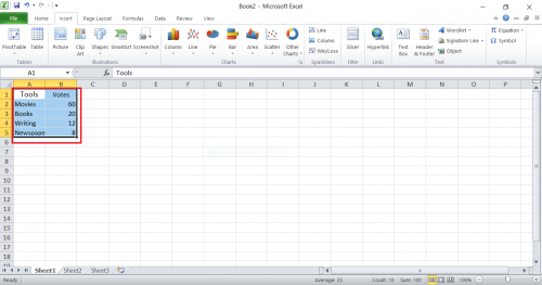
4. Click Insert > Pie.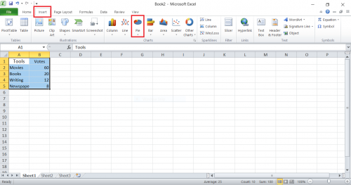
5. A pie chart will automatically appear.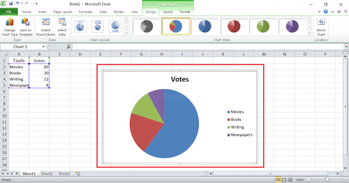
6. To enter the title of chart, click on highlighted area.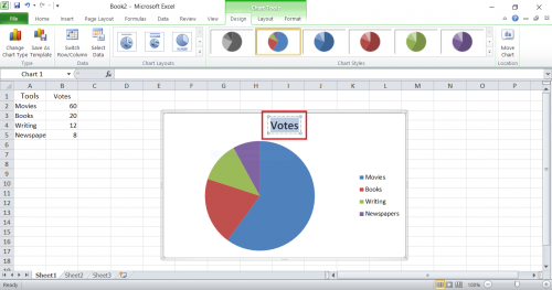
7. Enter your chart’s title.
Editing Your Pie-Chart
Labeling
1. The labels/values exist as automatically selected. Right-click anywhere on pie-chart > Format Data Labels.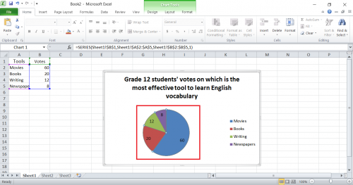
2. Label exists as simple numeric values (automatic).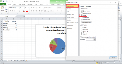
3. Select desired label. Click Close.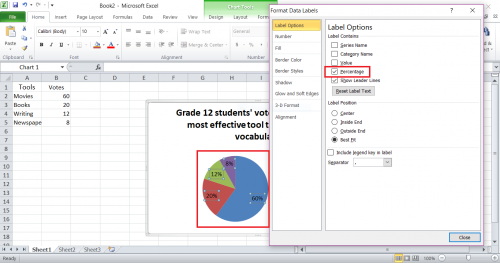
Editing Slices
1. To edit slices in pie-chart, right-click anywhere on chart > Format Data Series.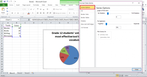
2. To shift angle of a slice, set rotation angle by entering value or moving blue cursor. Click Close, when done.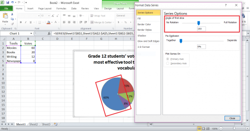
3. To separate slices in pie-chart, set the Together distance.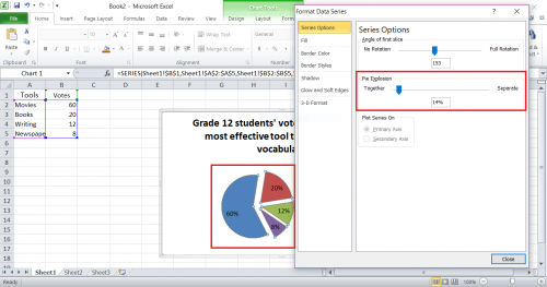
Changing Color
1. To change color of slices, select Fill. It is automatically selected.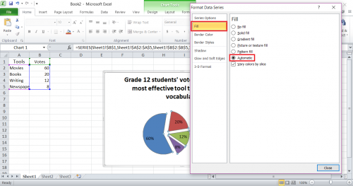
2. Select desired style of filling slices. Use color gradient to select color.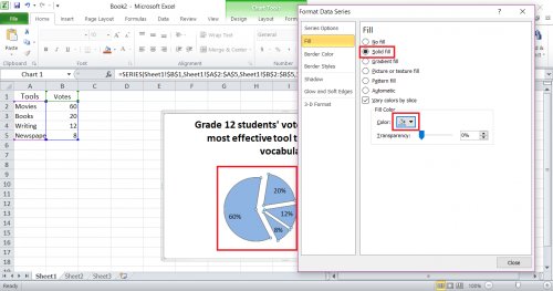
3. Right-click > Format Legend. It has automatically been set to left so it is present on the left.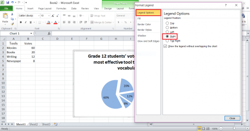
4. Right-click > Format Legend. Select desired position for legend. Click Close after finishing.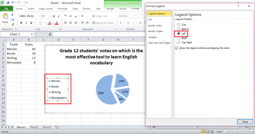
5. Select Fill to select options for filling legend box. It has automatically been set to No Fill.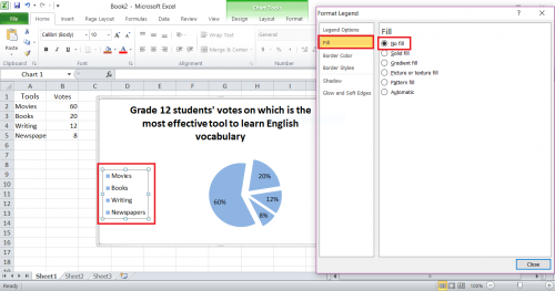
6. Select desired filling option for legend. Use color gradient for selecting color to fill legend with.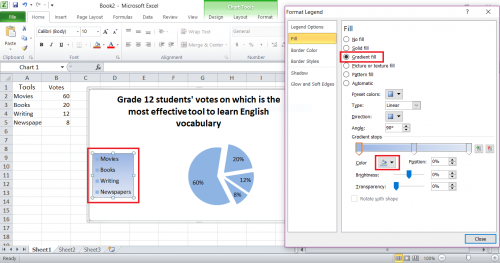
Changing Designs
1. To change chart’s design, click Chart Tools > Design.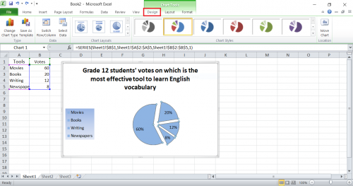
2. Select the desired design.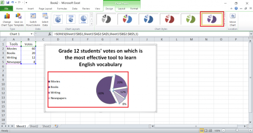
Changing Layouts
1. To change chart’s layout, regarding position of legend, select Chart Layout under Design.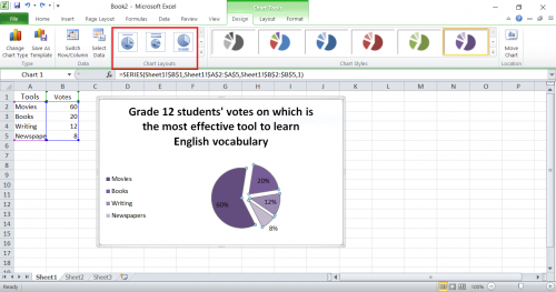
2. Choose the desired layout. Legends will shift position depending on layout chosen.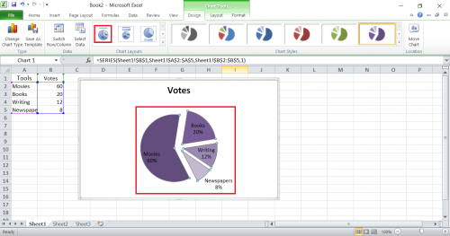
3. Chart title can also be entered by selecting Chart Tools > Layout > Chart Title.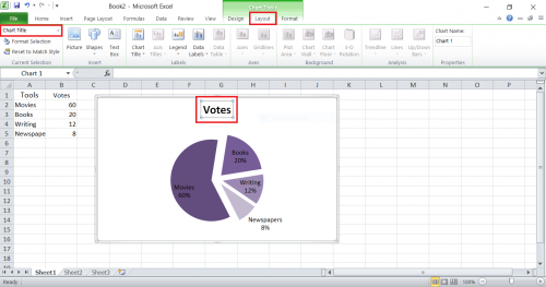
4. All the formatting done via right-clicks as shown above can also be done from Chart Tools > Layout > Format Selection.
Changing the Position of your Pie Chart
1. To change position of data labels, click Chart Tools > Layout > Data Labels.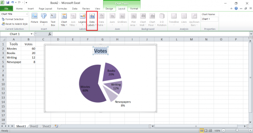
2. Set the desired data label from drop-down options (outside end shown here).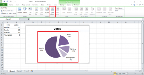
Formatting Slices
1. Slices can also be formatted under Chart Tools > Format.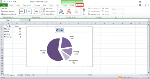
To format slices, select Shape Effects. Select desired shape effect from the drop-down options (shadow effect illustrated below).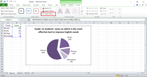
2. To access more shape effects, right-click slice to be formatted > Format Data Points > Shadow. Use Presents for shading area and Color to change shade’s color.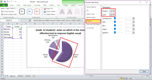
Applying 3-D effects
1. To give 3-D effects to slices, select 3-D Format. Use top to give 3-D effect on slice’s top, and so on.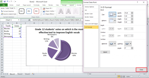
2. Hit close after finishing.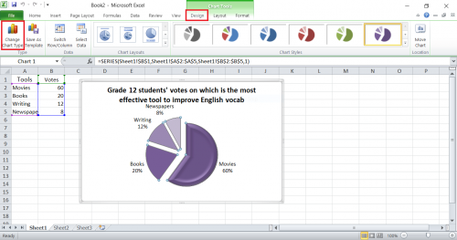
Changing Chart Type
1. To change chart type, select Chart Tools > Design > Change Chart Type.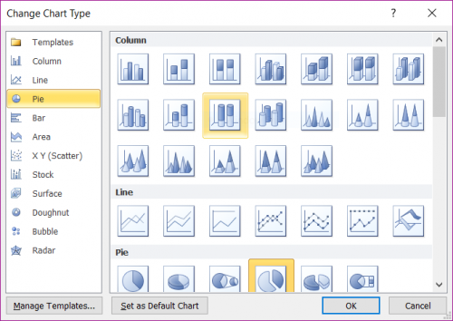
2. Select desired chart type. Click OK.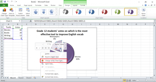
You can also add a trendline to a chart.
Chart type can also be changed by right-clicking > Change Series Chart Type.

