Excel 2013: Find Duplicate Data Using Conditional Formatting

Finding duplicate data within an Excel worksheet is a difficult task to attempt to do manually. Conditional formatting techniques can highlight this duplicated data to facilitate easier removal.

Excel documents can get notoriously huge. Often this is due to duplicated and repeated data. Finding and removing this data can be mind-numbingly boring and painful. Some research secretaries have entire careers of just staring at the data in Excel trying to discover and remove duplicate row entries. Accidental repeated imports are common culprits in this situation.

This tech-recipe tutorial will introduce you to removing duplicate data through conditional formatting. Instead of having to manually scan for data, these steps will show you how to isolate your duplicated entries.

These techniques can be expanded to a wide range of data; however, we will start with the simple case of duplicated entries in a list.

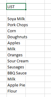
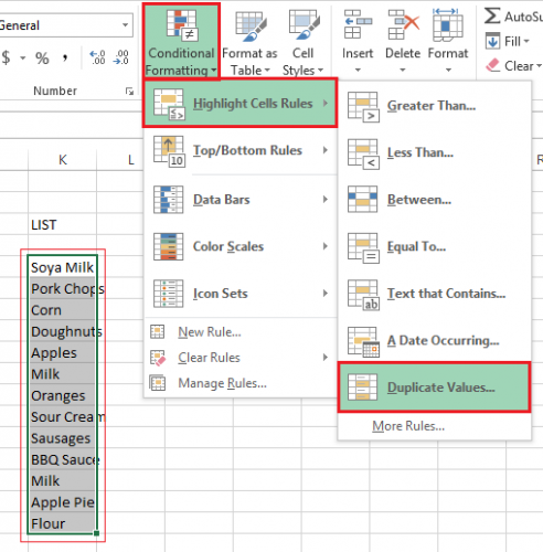
1.Highlight the list which you are going to search for duplicates. 

2.From the Excel ribbon select Conditional Formatting, then choose Highlight Cells Rules, and finally click on Duplicate Values. 

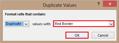
3.Under Duplicate Values select the format that you like best. For this tutorial I chose Red Border. After you have adjusted your settings click OK. 

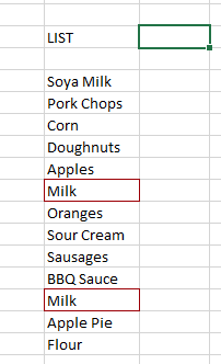
Now your duplicate entries will be highlighted. This highlighted data can be examined to see if it should be removed.

In a research environment, for example, this is one of the reasons for using unique IDs for samples. If these unique IDs are highlighted suggesting duplication, then the redundant data can be identified and removed.