
I was working in Google Sheets creating a dashboard that summarized data in another sheet. Specifically, I was trying to make a table that showed a list of each client that owed money. I tried to do this with a pivot table, but for some mysterious reason, pivot tables in Google Sheets do not automatically update. Because of this, it did not reflect changes in my source data until I manually updated the pivot table. That is when I discovered Google Sheets Filter function.
Using the Google Sheets Filter function was actually a pretty big deal for me, since there is no Excel equivalent. With the Filter function, you simply type your filter equation into the top cell of your summary table, and Google Sheets will fill in the cells beneath it with all the values that meet your criteria. In my case, I filtered client names that had an amount due greater than $0. The strange thing is that the formula only exists in the first cell – the cells underneath only have the text that was looked up from your source data. You can add, delete, and edit the source data, and the filter function will automatically update.
Here is my setup. Sheet 2 is my source data. It looks like this: 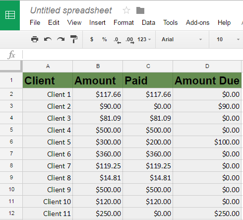
I will enter my formula in Sheet 1 cell A2. It ends up looking like this: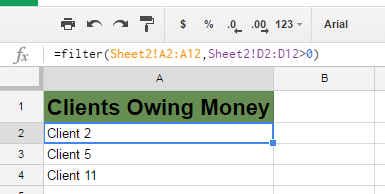
1.The format of the function is as follows:
=filter(range, condition 1, [condition 2]…)
My range is the cells containing the client names, and my only condition is that the associated amount due in Column D is >0. In my formula, Sheet2!A2:A12 is the range of cells I want to look through and filter into my Sheet 1 table. Sheet2!D2:D12>0 is where I say that the cell in Column D (my Amount Due) is greater than 0.
My formula is =filter(Sheet2!A2:A12,Sheet2!D2:D12>0).
2.Now, what if you want to get fancier and return multiple columns from your source data? Change the range in your formula to Sheet2!A2:D12 to return all four columns of data that match the filter criteria.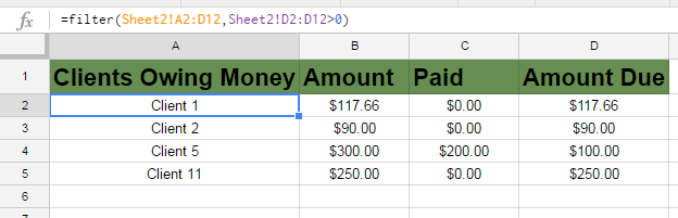
3.If you get a #REF! error, it is probably because you did not leave enough space for the filter function to fill in all the rows it wants to return. You need to leave plenty of space for it to do its thing. 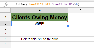
Note: If you are trying to use the Google Sheets filter function to get a list of unique values from a range, you want to use the Unique function. Check out my article on that topic here.

