
Dealing with an enormous amount of data is hard in itself. Excessive scrolling and managing rows and columns is a frustrating ordeal, to say the least. However, learning how to freeze panes in Excel is one way of slicing this ordeal into a manageable difficulty.
For one, it saves you from the hassle of scrolling all over the Excel spreadsheet just to locate your column and row headers. This is a huge problem when you have stacks and stacks of rows and columns and are finding it hard to navigate the Excel spreadsheet you’re currently working on.
Also, this little Excel trick will shoot your productivity through the roofs. It’s something you should absolutely know if your work involves confrontation with Microsoft Excel on a daily basis.
Note: It’s noteworthy to mention here that it is not possible to lock or freeze individual cell references in a single place.
How to Freeze panes in excel with Visual instructions
How to Freeze Topmost Rows and Columns in Excel
To Freeze topmost rows and columns in Excel, you don’t have to do anything at all, tbh. There’s an ib-build feature that makes the job a piece of cake for you.
To access this feature, go to the View tab, select Freeze Panes, and Select either Freeze top rows or columns, according to your preferences.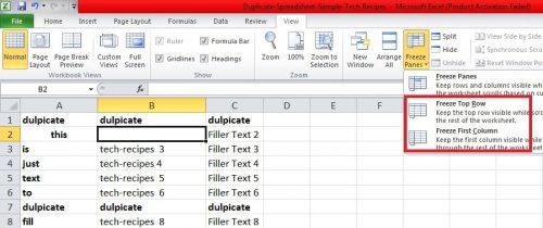
Step-by-Step: How to Freeze Rows in Excel
Okay, so there are manual ways of freezing rows and columns in excel, but we’re not going to be talking about them because they’re not as effective as the built-in Freeze panes feature in Excel.
To make sure that you don’t lose sight of your columns and headers, here’s what you have to do.
1. Open Your Excel Spreadsheet.
2. Select the row right underneath the row you want to freeze. In this case, I want to freeze the second row, so I’m selecting the third row.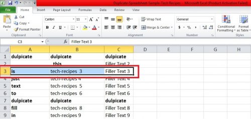
3. At the top of your Excel window, go to the View Tab.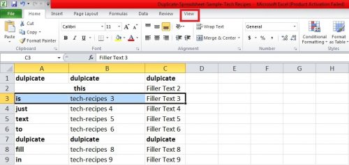
4. Tap Freeze Panes, and from the drop-down menu, select Freeze Panes.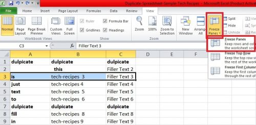
And this is how simple it is. You can now scroll down or across your spreadsheet without having to remind yourself the contents of these rows.
How to Freeze Columns in Excel
1. Select the first cell to the right of the column you want to freeze. In this case, I want to freeze the first Column A so, I’m going to select the cell B2.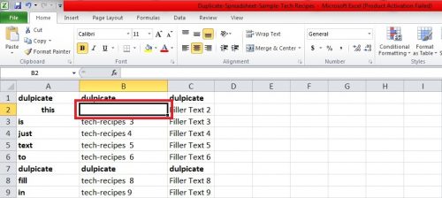
2. Open the View tab.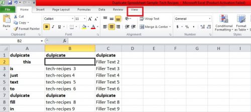
3. Go to Freeze panes> Freeze panes.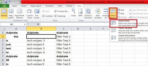
How to Freeze Columns and Rows at the Same Time
1. Microsoft Excel also gives you the option to freeze both rows and columns at the same time. In order to this, you have to follow a similar pattern, with a slight modification.
2. To lock rows and column at the same time, locate the cell that is right underneath and right to the columns you want to freeze. For example, if you want to loc the first column and the first row, select the cell reference B2.
Then, follow the same pattern that you will in the case in the case of individual columns and rows