Excel 2013: Create Progress Bars

Using Excel 2013’s conditional formatting features, you can create progress bars on your spreadsheets. Progress bars are used to graphically represent the advancement of the data. Essentially, you get a chart-like effect within the rows and cells themselves.

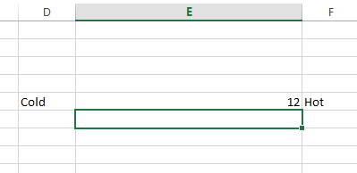
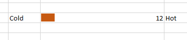
Below is an example of the setup that you should have before you start. I will use Cold/Hot as my demonstration. I also stretched the E cell to make the progress bar longer. This is done to see a more accurate bar, but this step is not a requirement. As you can see, I put the number 12 in the progress bar cell. This number will be the percentage of the bar that is shaded.

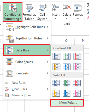
From the Excel ribbon, select Conditional Formatting and then Data Bars. Next, select More Rules.. 

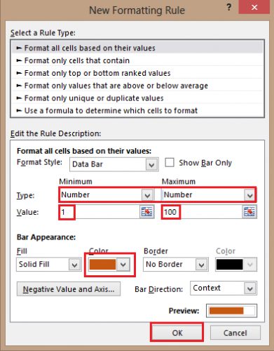
Now, you should see a window which will allow you to create a new formatting rule. For this step, we want to adjust the settings as follows: 

Type: Chose Number, both Minimum and Maximum.

Value: Set the Minimum value to 1 and the Maximum value to 100. 

Finally, chose your color, and click OK.

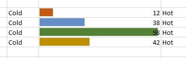
If you have adjusted all of the previous settings correctly, you should now see a progress bar.

Below are some examples with various values.