
If you work in more than one language with Excel, then you probably have noticed that you have problems converting dates from the European format (dd/mm/yyyy) to the American English format (mm/dd/yyyy). In fact, in most countries outside the US, the date is written as dd/mm/yyyy. (i.e., The day is first, the month is next, and the year is at the end.) If you download a document from your bank or if someone sends you an email with a spreadsheet in TXT, HTML, or CVS format, the dates will be backwards when you import it into the English language of Excel. You would have the same problem going from US English to another Latin-based language. Fortunately, converting the date format dd/mm/yyyy to mm/dd/yyyy is simple. Read on to find out how.
If you installed Microsoft Excel 2013 USA English version, when you open a file store in European or Latin American formats, Excel will not recognize the dates. Therefore, you could not apply a date format. You could not convert, for example, 01/10/2014 to 10 October 2014. If someone sent you a document that is already saved in spreadsheet format, you will not have any problem going from one language to another.
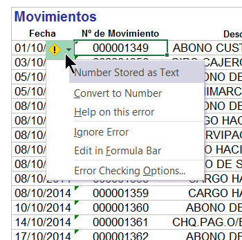
Here is an example. The spreadsheet below was downloaded in HTML format from a Spanish bank website. The dates are written in dd/mm/yyyy format.
1.The way to change this is to take the string of text, for example, 01/10/2014 and convert it to 10/01/2014. Then plug that into the Date() function in Excel.
Even Excel is complaining about this example. It tells you that it has stored the text as a number (Excel considers dates as numbers.).
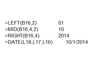
2.To fix this, use the LEFT, MID, RIGHT, and DATE functions:
LEFT—This takes the characters from the left. Below we wrote =LEFT(B16,2), meaning take the first two letters from the date located at cell B16.
MID—Here you tell it where to start to take letters from the middle. So =MID(B16,4,2) means start at position 4 and then take the two characters there. You start at 4 because the first three characters are the date and the slash (/).
RIGHT—This is the opposite of left. Here =RIGHT(B16,4) means we tell it to take the last four characters. The example below shows the formula and the end result.
Note that you could have written the formula all in one cell, but it would he harder to read. However, doing that saves you from using up a whole column for each individual step in the formula.
3.Now, you can work with the date like you would want, doing things like sorting the data by date and doing date math (e.g., adding 1 to the date to get the next day and formatting it it to say “October 1, 2014”).

